# load the packages
library(readr)
library(tidyverse)
library(gganimate)
library(dplyr)
library(magrittr)

# load the data
climate <- read_csv("climate_spending.csv")

energy <- read_csv("energy_spending.csv",
                    col_types = cols(year = col_integer()))

federal <- read_csv("fed_r_d_spending.csv")
Even though I can go further and do an investigative plotting from the rest data it is not done here. I was more focused on the scientific notation values in the plotting and scales, which were bothering me a lot.
3 Data sets are given here, they are
- Global Climate Change Research Program Spending. - climate
- Energy Departments Data. - energy
- Total Federal R & D Spending by Department. - federal
Oddly though climate data-set did not have year values, I checked the downloaded csv file and the GitHub upload as well. Well, that did not stop me from doing some tidy plotting.
You can obtain the data from here. It should be noted that I am not going to rename the abbreviation of departments with their full names, so below is a screen shot which would come in handy.
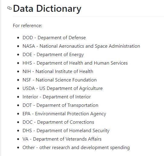
Department Full Names with Abbreviations
Scientific notation of numbers and plotting them was fun. Except for the R and D budget, other 3 have a steady increase over the years. Further, the R and D budget is very small than the others. Code: https://t.co/jmzfTGMRaT #tidytuesday pic.twitter.com/3WfBU72kWW
— Amalan Mahendran (@Amalan_Con_Stat) February 12, 2019
Climate Change Research
As I mentioned earlier for the climate data there are no values in the year column, but according to summary I was able to deduce that we have 18 years of information. When we do plot it is going to be the summation for each department in a bar.
Clearly NASA has the most amount ( above than 2.5 x 10^10 USD) of spending because rockets are expensive, second place goes to NSF (5 x 10^9 USD) and third place to NOAA. Lowest amount of spending is to the Department of Interior (8.47 x 10^8 USD).
ggplot(climate,aes(x=fct_inorder(department),y=gcc_spending,fill=department))+
  geom_bar(stat="identity",show.legend = FALSE)+
  ggtitle("Total GCC Spending for 18 Years")+
  scale_y_continuous(labels = scales::scientific,breaks = seq(0,2.75e+10,0.25e+10))+
  xlab("Sub Agency / Department")+ylab("GCC Spending (in USD)")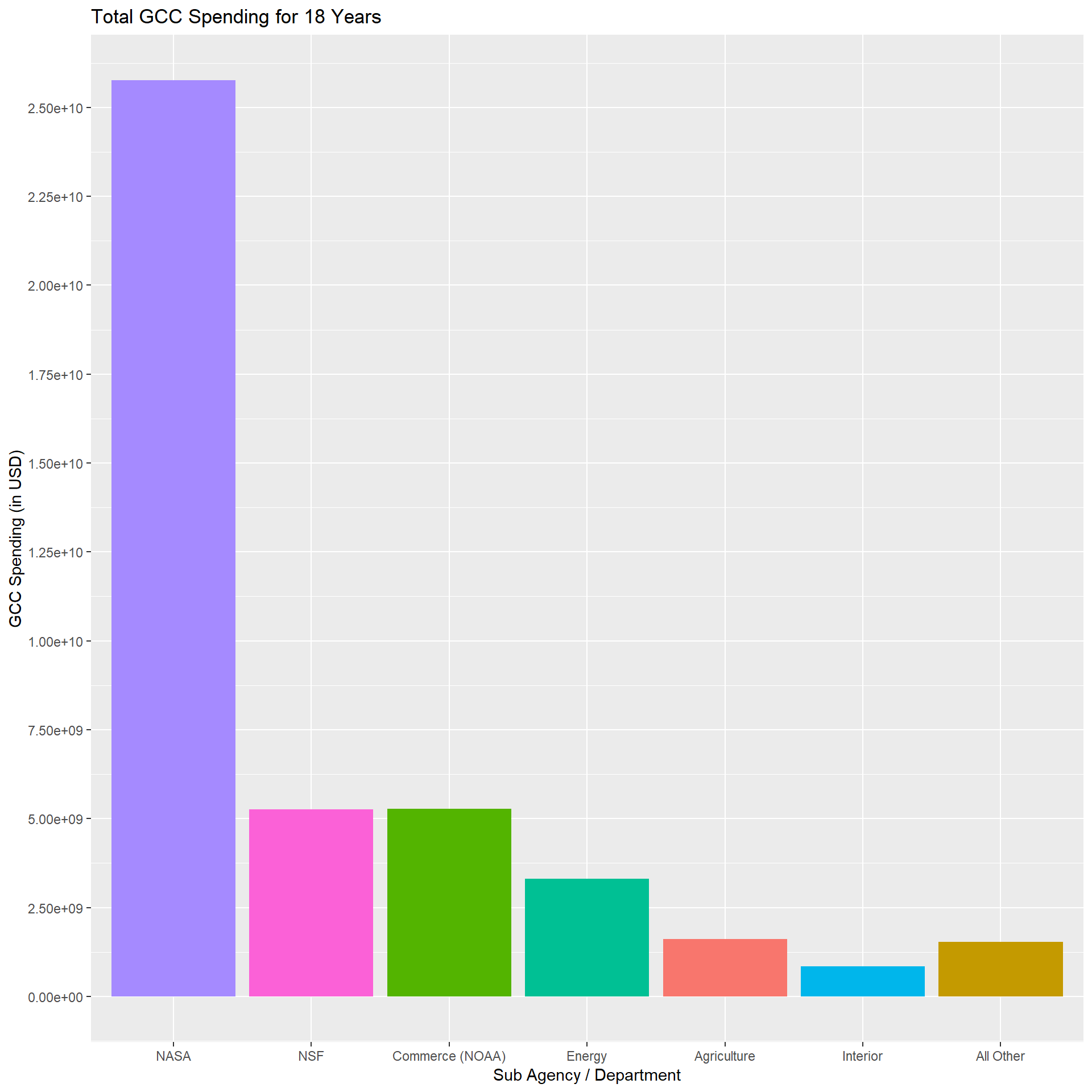
Energy
Since 1997 to 2018 how Energy Department funding has changed with sub agency/ department is the purpose of the below bar plot. Office of Science R & D and Atomic Energy Defense are competitive over the years and for a short period of time the latter has less funding than the former, this was between 2006 to 2010.
Other agencies oscillates over the years while reaching new highs and lows.
p<-ggplot(energy,aes(x=department,y=energy_spending,fill=year))+
          geom_bar(stat="identity",position ="identity")+
          transition_time(year)+
          geom_text(aes(label=scales::scientific(energy_spending)),
                    vjust = "inward", hjust = "inward")+
          ease_aes("linear")+coord_flip()+
          ylab("Energy Spending (in USD)")+
          theme(legend.position = "right")+
          xlab("Sub Agency / Department")+
          scale_fill_continuous(breaks = seq(1997,2018,3))+
          scale_y_continuous(labels = scales::scientific)+
          ggtitle("Energy Spending Of Year : {frame_time}")

animate(p,fps=1,nframes=22)
Federal
Data of Federal funding has four different types to be compared and they are mentioned below in the description image which would make explanation more easier.
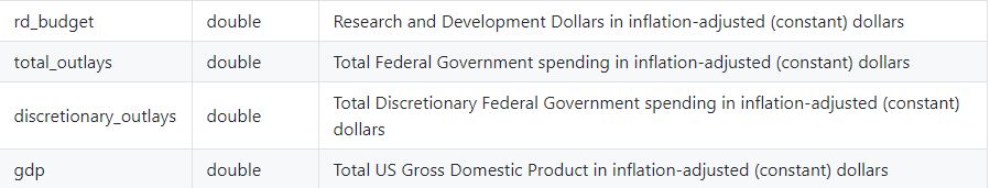
Except rd_budget others have a very clear increase in amount between 1976 to 2018. Further, all four plots have different scales and the limits are widely different for each plot.
p<-federal %>%
    gather(funding,amount,c(rd_budget,total_outlays,discretionary_outlays,gdp)) %>%
    ggplot(.,aes(x=factor(department),y=amount,color=year))+
           geom_jitter()+transition_time(year)+
           ease_aes("linear")+coord_flip()+
           shadow_mark()+
           theme(legend.position = "right")+
           ylab("Spending in USD")+xlab("Department")+
           ggtitle("Total Federal R&D for Year : {frame_time}")+
           scale_color_continuous(breaks = seq(1976,2018,6),labels=seq(1976,2018,6))+
           scale_y_continuous(labels = scales::scientific)+
           facet_wrap(~funding,scales = "free")

animate(p,fps=1,nframes=42)
THANK YOU