

- Claps
- Top 10 Authors and Claps for their posts
- Top 10 Authors with most posts
- Top 10 Authors who have posts with Images
- Top 10 Authors who have posts without Images
- Top 10 Authors and Reading time for their posts
- Top 5 Publications with most posts
- Word Cloud for the Titles from Top 10 Authors
- Word Cloud for the Titles from Top 5 publications
- Conclusion
- Further Analysis
#loading packages
#load data
library(readr)
#manipulate data
library(dplyr)
library(magrittr)
# format table with expense
library(formattable)
# knitting the document
library(knitr)
# another type of table
library(kableExtra)
# playing with strings
library(stringr)
# combining two plots
library(grid)
library(gridExtra)
# that theme you wanted
library(ggthemr)
# text analysis
library(tm)
library(SnowballC)
library(RColorBrewer)
library(wordcloud)

# adding theme called fresh for plots
ggthemr("fresh")
#loading the data
medium <- read_csv("medium_datasci.csv")
attach(medium)
Focusing on Claps with Authors and publications, where does writing alot of posts will get you with popularity and claps. The code will focus on Top 10 Authors with most of the posts and Claps they have received. Further, does having an image in the post matter ?. Finally, word clouds for Top 10 authors and Top 5 publications with their titles.
my take medium posts on week 36 #tidytuesday https://t.co/FTAZh0vKI8
— Amalan Mahendran (@Amalan_Con_Stat) December 8, 2018
Claps
Table indicates that 25,729 posts have 0 claps, while 7,093 posts with only one clap, and finally 3044 posts with 2 claps. The only odd one is posts with 50 claps where the count is 970.
# extracting the top 15 with most claps
claps_table<-table(claps) %>%
                     sort() %>%
                     tail(15)

# table it up
kable(t(claps_table),"html") %>%
  kable_styling(bootstrap_options = "striped",full_width = T) %>%
row_spec(0,bold = T,font_size = 13,color = "grey")| 13 | 12 | 9 | 8 | 11 | 7 | 50 | 10 | 6 | 5 | 4 | 3 | 2 | 1 | 0 |
|---|---|---|---|---|---|---|---|---|---|---|---|---|---|---|
| 602 | 634 | 661 | 721 | 759 | 864 | 970 | 989 | 1124 | 1389 | 1402 | 2150 | 3044 | 7093 | 25729 |
Top 10 Authors with most posts
Yves Mulkers has most amount of posts with 487 but only 3,779 claps. This is not the case for Corsairs publishing where for 156 posts the number of claps are 111,501. Even looking at other authors names we can see that writing alot of posts does not create claps.
# finding who are the top 10 authors with claps
# summary.factor(medium$author) %>%
#  sort() %>%
#  tail(11)

# extracting posts only from the top 10 authors with most posts
Top10_author<-subset(medium,
       author =="C Gavilanes" | author == "Jae Duk Seo" |
       author == "Corsair's Publishing" | author=="Alibaba Cloud" |
       author == "Ilexa Yardley" | author == "Peter Marshall" |
       author == "AI Hawk" | author == "DEEP AERO DRONES" |
       author == "Synced" | author == "Yves Mulkers")

# plotting the top 10 authors
g1_Top10_a<-ggplot(Top10_author,aes(x=author))+
            coord_flip()+ geom_bar()+
            xlab("Author")+ylab("Frequency")+
            ggtitle("Top 10 Authors and number of posts they have written")+
            geom_text(stat = 'count',aes(label=..count..),hjust=0.5)

# plotting the top 10 authors and their claps
g2_Top10_a<-Top10_author[,c("author","claps")] %>%
            group_by(author) %>%
            summarise_each(funs(sum)) %>%
            ggplot(.,aes(x=author,y=claps))+ geom_bar(stat = "identity")+
            ggtitle("Total number of Claps they got")+
            xlab("Author")+ylab("Claps")+
            coord_flip()+geom_text(aes(label=claps),hjust =0.5 )

# plotting two plots at same grid
grid.arrange(g1_Top10_a,g2_Top10_a,ncol=1)
Top 10 Authors who have posts with Images
Extracting the top 10 authors with posts which have images it is clear most of the posts do have Images and they do generate claps. This is true for Corsairs’s Publishing. With 154 posts it generates 109,906 claps. There are authors who have written more posts than totally received claps . It should be noted that two Authors did not add any Images for their post and they are Peter Marshall and C Gavilanes.
# plotting top 10 authors with Image
I1_g1_Top10_a<-subset(Top10_author[,c("author","image")],image==1) %>%
            ggplot(.,aes(x=author))+ geom_bar()+coord_flip()+
            xlab("Author")+ylab("Frequency")+
            ggtitle("Top 10 Authors and posts which has Images")+
            geom_text(stat='count',aes(label=..count..),hjust =0.5 )

# plotting the claps for top 10 authors with Image
I1_g2_Top10_a<-subset(Top10_author[,c("author","claps","image")],image==1) %>%
               group_by(author,image) %>%
               summarise_each(funs(sum)) %>%
               ggplot(.,aes(x=author,y=claps))+ geom_bar(stat = "identity")+
               coord_flip()+
               xlab("Author")+ylab("Claps")+
               ggtitle( "Total number of Claps they got")+
               geom_text(aes(label=claps),hjust =0.5 )

# top plots one grid
grid.arrange(I1_g1_Top10_a,I1_g2_Top10_a,ncol=1)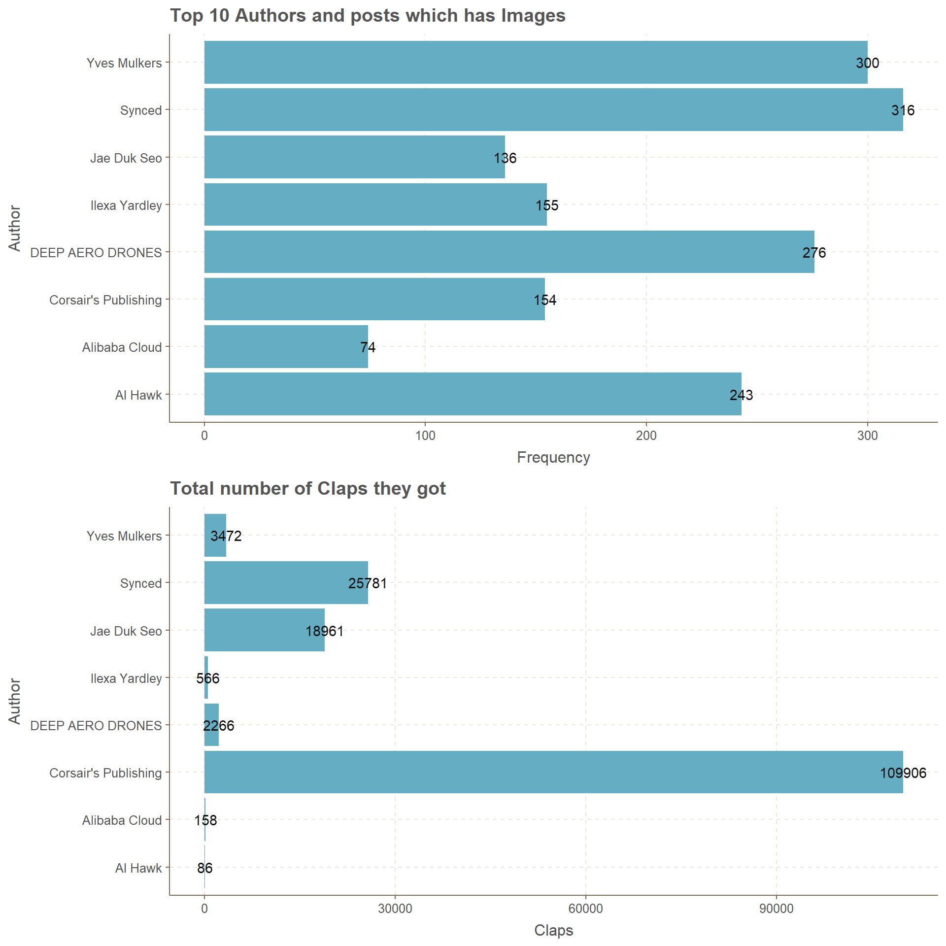
Top 10 Authors who have posts without Images
Posts without images have very low amount of total claps. To be specific 14 posts by Jae Duk Seo have 1833 claps but 2 posts by Corsair’s publishing has 1595 claps. That is very Impressive. Further there are even posts which have claps less than 10 where the number of posts is less than 5.
# plotting top 10 authors with No Image
I0_g1_Top10_a<-subset(Top10_author[,c("author","image")],image==0) %>%
               ggplot(.,aes(x=author))+ geom_bar()+coord_flip()+
               xlab("Author")+ylab("Frequency")+
               ggtitle("Top 10 Authors and posts without Images")+
               geom_text(stat='count',aes(label=..count..),hjust =0.5 )

# plotting the claps for top 10 authors with No Image
I0_g2_Top10_a<-subset(Top10_author[,c("author","claps","image")],image==0) %>%
               group_by(author,image) %>%
               summarise_each(funs(sum)) %>%
               ggplot(.,aes(x=author,y=claps))+ geom_bar(stat = "identity")+
               coord_flip()+
               xlab("Author")+ylab("Claps")+
               ggtitle("Total number of claps they got")+
               geom_text(aes(label=claps),hjust =0.5 )

# top plots one grid
grid.arrange(I0_g1_Top10_a,I0_g2_Top10_a,ncol=1)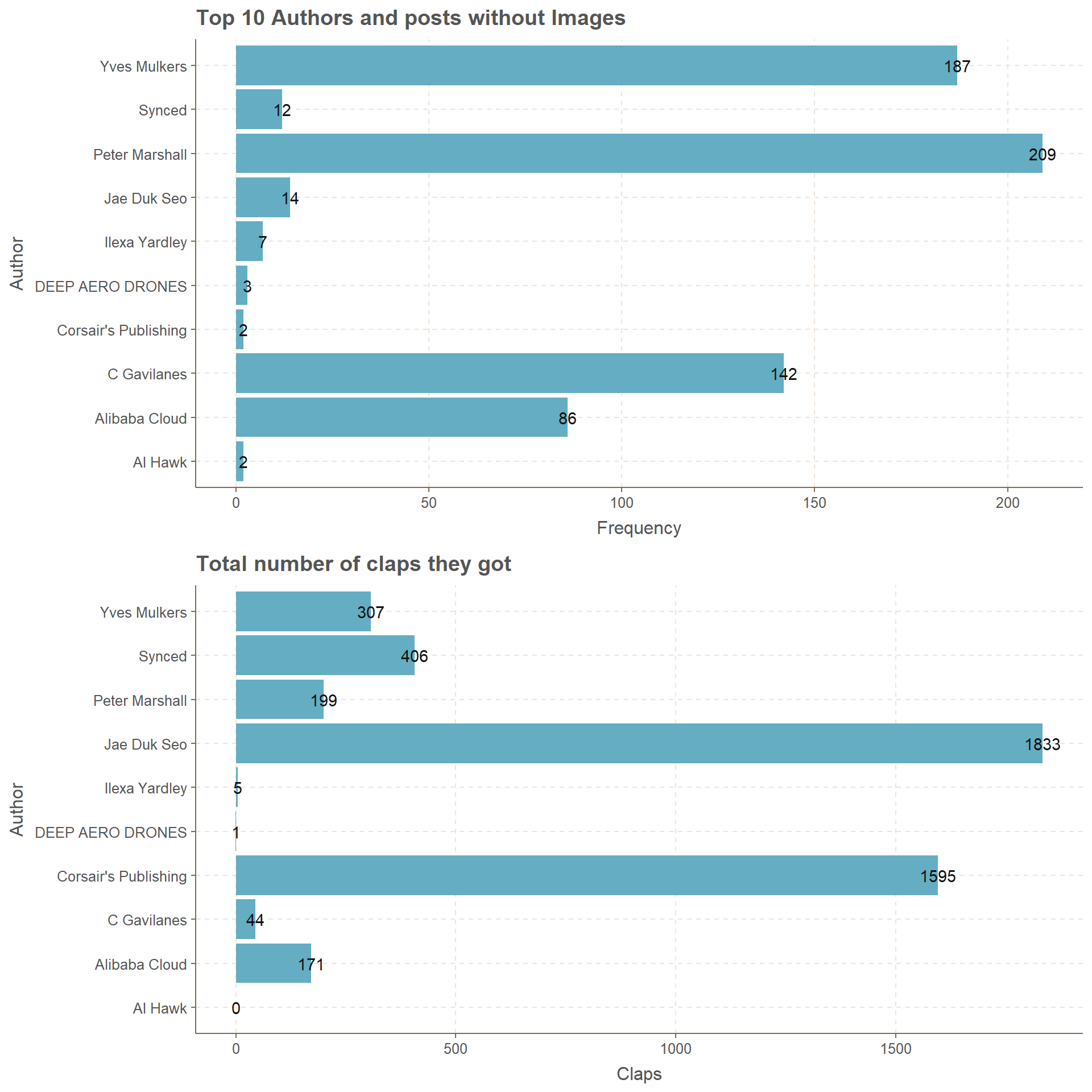
Top 10 Authors and Reading time for their posts
Reading in minutes, does it has anything to do with number of posts?. Looking at the plot it is clear that posts from Synced has more total reading time than Yves Mulkers with highest number posts. The difference between posts is close 150, while difference between reading times is above 150 for Yves Mulkers and Synced.
# plotting top 10 authors with reading times
RT_g1_Top10_a<-Top10_author[,c("author","reading_time")] %>%
            group_by(author) %>%
            summarise_each(funs(sum)) %>%
            ggplot(.,aes(x=author,y=reading_time))+ geom_bar(stat = "identity")+
            ggtitle("Reading Time")+
            xlab("Author")+ylab("Reading Time in minutes")+
            coord_flip()+geom_text(aes(label=reading_time),hjust =0.5 )

# printing the above plot with number of posts
grid.arrange(g1_Top10_a,RT_g1_Top10_a,ncol=1)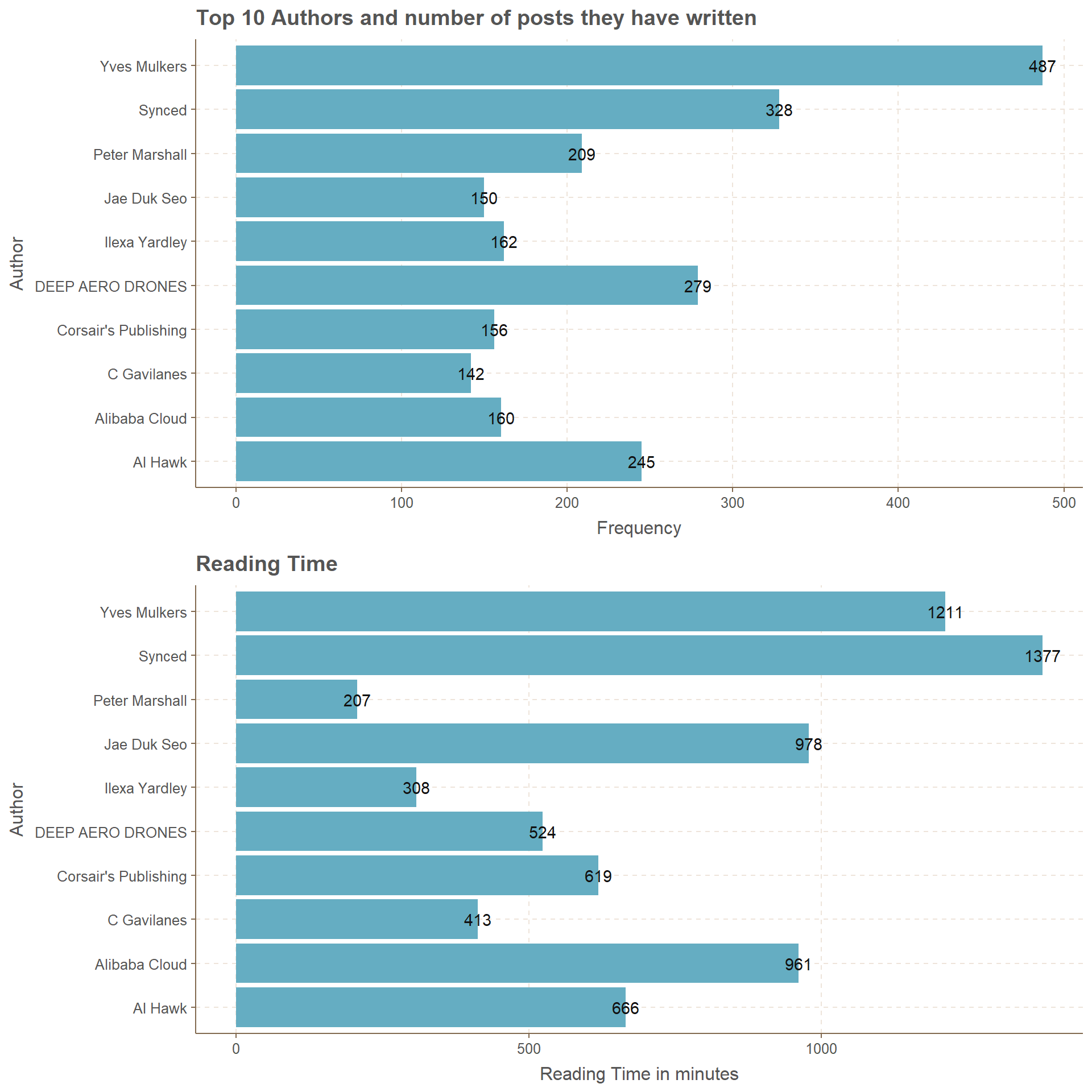
Top 5 Publications with most posts
Publications with most number of posts has the highest number of claps and order achieved
in the “Top 5 publications and number of posts they have written” plot is maintained in the “Total number of Claps they got” plot as well. This simply refers, when you write alot of posts under a publication you will receive alot of claps because of the foundation these specific publications holds in Medium.
# finding who are the top 5 publications with claps
# summary.factor(medium$publication) %>%
#  sort() %>%
#  tail(11)

# extracting posts only from the top 5 publications with most posts
Top5_pub<-subset(medium,
       publication =="Towards Data Science" |
       publication == "Hacker Noon" |
       publication == "Becoming Human: Artificial Intelligence Magazine" |
       publication =="Chatbots Life" |
       publication == "Data Driven Investor" )

# plotting the top 5 publications
g1_Top5_p<-ggplot(Top5_pub,aes(x=str_wrap(publication,15)))+
            coord_flip()+ geom_bar()+
            xlab("Publication")+ylab("Frequency")+
            ggtitle("Top 5 Publications and number of posts they have written")+
            geom_text(stat = 'count',aes(label=..count..),hjust=0.5)

# plotting the top 5 publications and their claps
g2_Top5_p<-Top5_pub[,c("publication","claps")] %>%
            group_by(publication) %>%
            summarise_each(funs(sum)) %>%
            ggplot(.,aes(x=str_wrap(publication,15),y=claps))+
            geom_bar(stat="identity")+
            xlab("Publication")+ylab("Claps")+
            ggtitle("Total number of Claps they got")+
            coord_flip()+geom_text(aes(label=claps),hjust =0.5 )

# plotting two plots at same grid
grid.arrange(g1_Top5_p,g2_Top5_p,ncol=1)
Word Cloud for the Titles from Top 10 Authors
Word cloud from the titles of the posts by Top 10 authors of most number of posts is below. The words thing, read, data, drone and new are with highest mentions. Where words such as big, telecom and tech are next in the line with higher amount of posts. In restrictions I have considered that this word cloud will have 1500 words and only if a word atleast holds the frequency of 10.
Well, I could clearly see that there cannot be 1500 words here.
#convert into data frame
Top10_author<-data.frame(Top10_author)

# Calculate Corpus
Top10_author.Corpus<-Corpus(VectorSource(Top10_author$title))

# clean the data
Top10_author.Clean<-tm_map(Top10_author.Corpus,PlainTextDocument)
Top10_author.Clean<-tm_map(Top10_author.Corpus,tolower)
Top10_author.Clean<-tm_map(Top10_author.Clean,removeNumbers)
Top10_author.Clean<-tm_map(Top10_author.Clean,removeWords,stopwords("english"))
Top10_author.Clean<-tm_map(Top10_author.Clean,removePunctuation)
Top10_author.Clean<-tm_map(Top10_author.Clean,stripWhitespace)
Top10_author.Clean<-tm_map(Top10_author.Clean,stemDocument)

# save as png
#png(filename = "wordcloud1.png",width = 1024,height = 768)
# plot the word cloud
wordcloud(Top10_author.Clean,max.words = 1500,min.freq = 10,
          colors = brewer.pal(11,"Spectral"),random.color = FALSE,
          random.order = TRUE)
Word Cloud for the Titles from Top 5 publications
This word cloud also has similar restrictions for number of words and minimum frequency for a word. Words such as data, learn, use, machin, network, deep, scienc and artifici have most amount of frequency. Further, words such as neural, intellig, chatbot, part and python are also with significant amount of frequency. Here we can see clearly see there can be more than 1000 words.
#convert into data frame
Top5_pub<-data.frame(Top5_pub)

# Calculate Corpus
Top5_pub.Corpus<-Corpus(VectorSource(Top5_pub$title))

#clean the data
Top5_pub.Clean<-tm_map(Top5_pub.Corpus,PlainTextDocument)
Top5_pub.Clean<-tm_map(Top5_pub.Corpus,tolower)
Top5_pub.Clean<-tm_map(Top5_pub.Clean,removeNumbers)
Top5_pub.Clean<-tm_map(Top5_pub.Clean,removeWords,stopwords("english"))
Top5_pub.Clean<-tm_map(Top5_pub.Clean,removePunctuation)
Top5_pub.Clean<-tm_map(Top5_pub.Clean,stripWhitespace)
Top5_pub.Clean<-tm_map(Top5_pub.Clean,stemDocument)

# save as png
#png(filename = "wordcloud2.png",width = 1024,height = 768)
# plot the word cloud
wordcloud(Top5_pub.Clean,max.words = 1500,min.freq = 10,
          colors = brewer.pal(11,"Spectral"),random.color = FALSE,
          random.order = TRUE)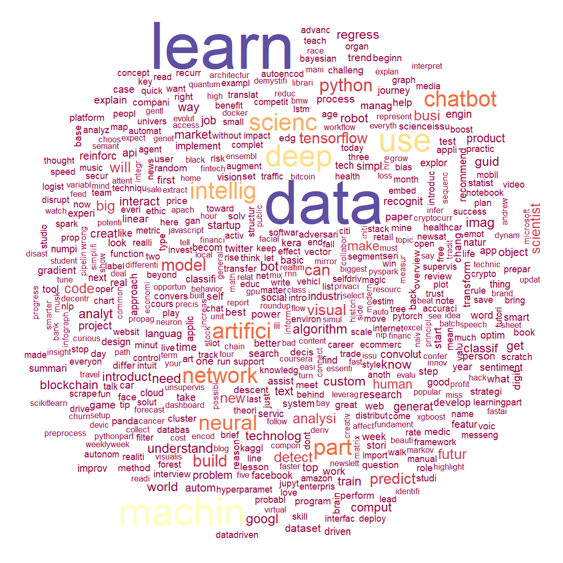
Conclusion
My conclusion of the above plots and tables in point form
Using dplyr to manipulate the data-set was useful when there is complication.
grid and gridExtra packages provide a safe way of combining multiple plots into one plot.
formattable and kableExtra were crucial in generating tables which are informative.
Word cloud or analyzing text is very useful and flexible when we use the above packages.
Further Analysis
Similarly we can do the above analysis for Top 5 publications and other variables.
Word clouds for subtitles also will be interesting to see, specially focusing on authors and publications.
Please see that
This is my sixth post on the internet so my mistakes in grammar and spellings should be very less than previous posts. I intend to post more statistics related materials in the future and learn accordingly. Thank you for reading.
THANK YOU