# load the packages
library(readr)
library(ggplot2)
library(lubridate)
library(ggthemr)
library(gridExtra)
library(magrittr)
library(knitr)
library(kableExtra)
library(readr)

# load the data
r_downloads_year <- read_csv("r_downloads_year.csv",
     col_types = cols(X1 = col_skip(), date = col_date(format = "%Y-%m-%d"),
                      time = col_time(format = "%H:%M:%S")))
r_downloads <- read_csv("r-downloads.csv",
     col_types = cols(X1 = col_skip(), date = col_date(format = "%Y-%m-%d"),
                      time = col_time(format = "%H:%M:%S")))
Week 31 : R and Package Downloads #TidyTuesday https://t.co/hALK5o4bGd
— Amalan Mahendran (@Amalan_Con_Stat) December 3, 2018
Introduction
Tidy Tuesday is a very good move to improve R programming for anyone who is interested in statistics. Data-sets are uploaded every Tuesday, and plots are published under the #tidytuesday. This is just me presenting a few accumulated plots for the data-set r-downloads.csv and r_downloads_year.csv.
I shall be focusing on the data set provided on 2018 October 30th, Which is R and Package download stats. My main objective is to understand how Sri Lankan users have behaved in this data-set.
The packages used in R are readr,ggplot2, lubridate, ggthemr, gridExtra, magrittr, knitr and kableExtra.
There are 701 downloads occurred in between the given time limit of 2017 October 20th to 2018 October 20th in Sri Lanka. Similarly, if we look at the downloads on the day of 2018 October 23rd, which is 3 observations. There are 7 variables to be concerned, which are
- date - date of download (y-m-d)
- time - time of download (in UTC)
- size - size in bytes
- version - R release version
- os - Operating System
- country - Two letter ISO country code
- ip_id - Anonymized daily ip code(unique identifier)
# extracting the observations only if the country is Sri Lanka
r_downloads_year_LK<-subset.data.frame(r_downloads_year,country=="LK")
r_downloads_LK<-subset.data.frame(r_downloads,country=="LK")

# number of observations
#dim(r_downloads_year_LK)
#dim(r_downloads_LK)
Operating Systems
Windows is not a favorable operating system for open source programming was my myth. Well, No longer I shall believe that if it is considering Sri Lankans and R programming.
#checking what type of operating systems are in use
ggthemr("flat dark")
ggplot(r_downloads_year_LK,aes(x=os))+geom_bar()+
    geom_text(stat='count', aes(label=..count..), vjust=-0.5)+
    xlab("Operating System")+ylab("Frequency")+
    scale_y_continuous(breaks=seq(0,675,by=25))+
    ggtitle("Operating system preference of Sri lankans for R",
              subtitle = "2017 October 20th - 2018 October 20th")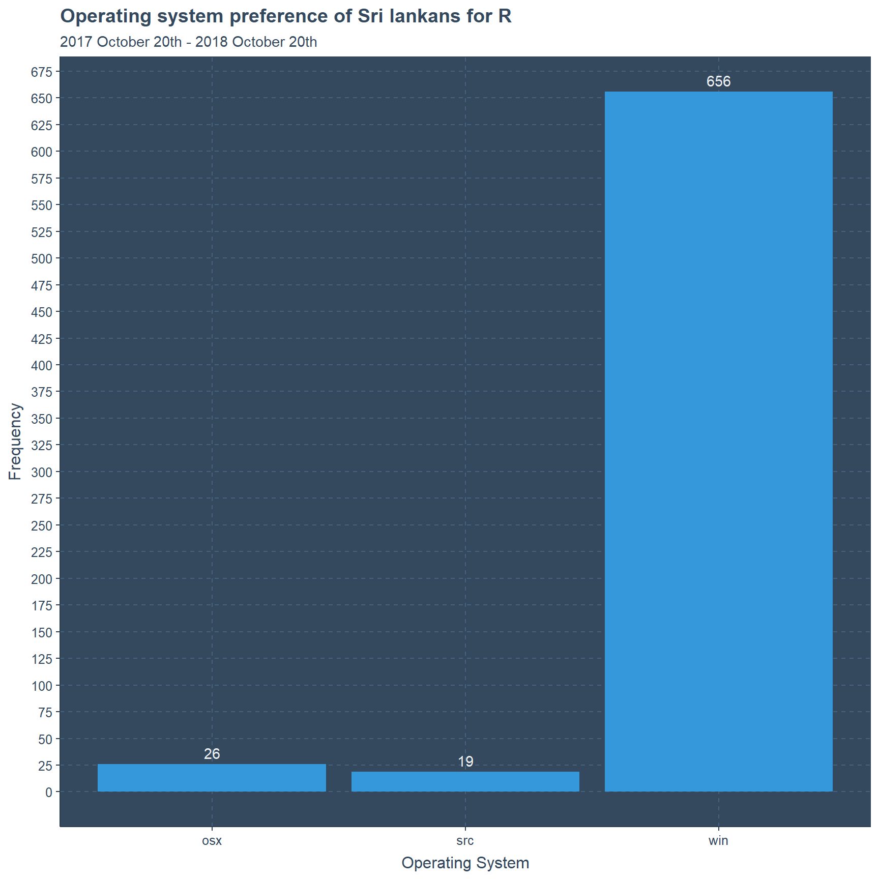
# frequency table for Operating system
tab1<-round(prop.table(table(r_downloads_year_LK$os)),4)
tab1<-as.data.frame(tab1)
names(tab1)<-c("Operating System","Frequency")
kable(tab1) %>%
  kable_styling(bootstrap_options = "striped", full_width = F,position="left") %>%
add_header_above(c("Frequency table to Operating system"=2))| Operating System | Frequency |
|---|---|
| osx | 0.0371 |
| src | 0.0271 |
| win | 0.9358 |
Majority of users have used Windows which is 93.58%, while Mac users are represented with 3.71% and finally 2.71% from the source file. Next, focusing on the R versions downloaded.
R versions
Versions are updated regularly for R and a grand update occurred on 2018 April for the version 3.5.0. Further, versions 3.4.3 and 3.4.4 were updated in the time gap considered. There are versions from 3.0.0 and higher for Sri Lankan users. It is crucial to study this where we can understand how far does the user have knowledge about R and updating the software version.
#checking what type of R versions were downloaded
ggplot(r_downloads_year_LK,aes(x=version))+geom_bar()+
    geom_text(stat='count', aes(label=..count..), vjust=-0.5)+
    xlab("R versions")+ylab("Frequency")+
    scale_y_continuous(breaks = seq(0,275,by=25))+
    ggtitle("R versions downloaded of Sri Lankans for R",
            subtitle = "2017 October 20th - 2018 October 20th")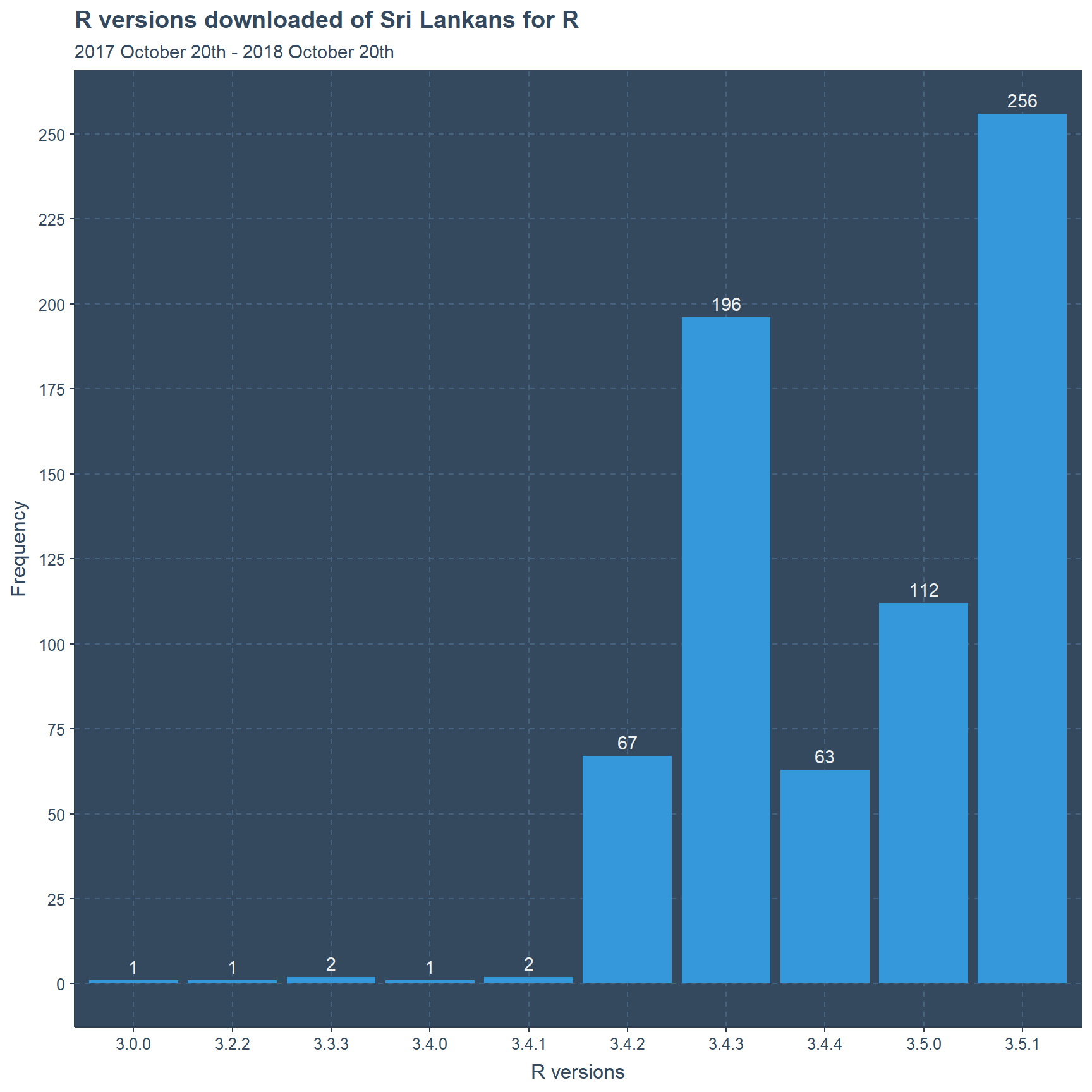
Table shows that version 3.5.1 represents a 36.52% followed by version 3.4.3 of 27.96% and in the third place version 3.5.0 with 15.98%. Further, all downloads are occurred for versions 3.0.0 or higher than it. People believed in 3.4.3 than 3.5.0, which could only mean that 3.4.3 was more stable for user and package requirements.
# frequency table to R versions
tab2<-sort(round(prop.table(table(r_downloads_year_LK$version)),4))
tab2<-as.data.frame(tab2)
names(tab2)<-c("R Version","Frequency")
kable(tab2) %>%
  kable_styling(bootstrap_options = "striped", full_width = F,position="left") %>%
add_header_above(c("Frequency table to R versions"=2))| R Version | Frequency |
|---|---|
| 3.0.0 | 0.0014 |
| 3.2.2 | 0.0014 |
| 3.4.0 | 0.0014 |
| 3.3.3 | 0.0029 |
| 3.4.1 | 0.0029 |
| 3.4.4 | 0.0899 |
| 3.4.2 | 0.0956 |
| 3.5.0 | 0.1598 |
| 3.4.3 | 0.2796 |
| 3.5.1 | 0.3652 |
If we further divide the operating systems bar plot with respective to R version it is clearly seen that only versions 3.5.1, 3.5.0, 3.4.4, 3.4.3 and 3.4.2 have maintained importance for the windows operating system.
# Checking what type of operating system is used with R version
#setting 10 colors becuase flat dark theme only has four originally
set_swatch(c("white","firebrick1","gold","darkorange","dodgerblue","darkblue",
             "forestgreen","green","grey","grey44","black"))
ggplot(r_downloads_year_LK,aes(x=os,fill=version))+geom_bar()+
  geom_text(stat='count',aes(y=..count..,label=..count..),position="stack",vjust=1)+
    xlab("Operating System")+ylab("Frequency")+
    scale_y_continuous(breaks=seq(0,675,by=25))+
    ggtitle("Operating system preference of Sri lankans for R",
              subtitle = "2017 October 20th - 2018 October 20th")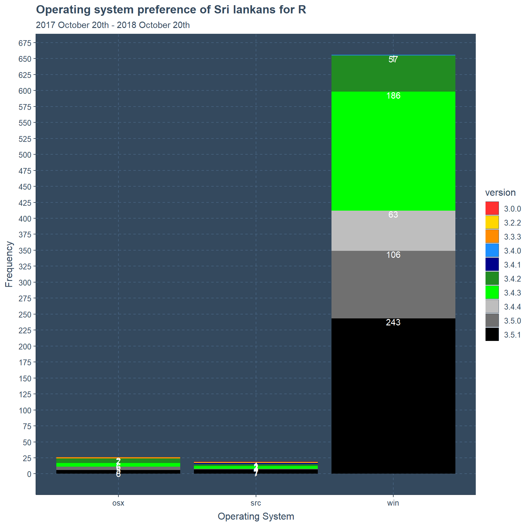
#Contingency table to R version versus operating System
kable(round(prop.table(table(r_downloads_year_LK$os,
                             r_downloads_year_LK$version)),4)) %>%
  kable_styling(bootstrap_options = "striped",full_width = T) %>%
add_header_above(c("Contingency table for R version vs Operating System"=11))| 3.0.0 | 3.2.2 | 3.3.3 | 3.4.0 | 3.4.1 | 3.4.2 | 3.4.3 | 3.4.4 | 3.5.0 | 3.5.1 | |
|---|---|---|---|---|---|---|---|---|---|---|
| osx | 0.0000 | 0.0000 | 0.0029 | 0.0000 | 0.0000 | 0.0100 | 0.0086 | 0.0000 | 0.0071 | 0.0086 |
| src | 0.0014 | 0.0014 | 0.0000 | 0.0000 | 0.0029 | 0.0043 | 0.0057 | 0.0000 | 0.0014 | 0.0100 |
| win | 0.0000 | 0.0000 | 0.0000 | 0.0014 | 0.0000 | 0.0813 | 0.2653 | 0.0899 | 0.1512 | 0.3466 |
Windows operating system percentages indicate that 34.66% of users have chosen version 3.5.1, 26.53% have chosen version 3.4.3 and finally version 3.5.0 with 15.12%. Close to 9% is represented by version 3.4.2 and 3.4.4.
Date versus Operating System
Date is a difficult variable in statistics therefore I have disseminated the date into 4 types, which are month(January to December), day(1-31), hour(0-23) and minutes(0-59). Further, I have tried to understand what type of operating systems were used in those time types.
#checking which months the downloads occured inrespecitive to operating system
ggthemr("flat dark")
ggplot(r_downloads_year_LK,aes(x=month(date),fill=os))+
    geom_bar()+ xlab("Months") +ylab("Frequency")+
    scale_y_continuous(breaks =seq(0,140,10))+
    scale_x_continuous(breaks=1:12) +
    ggtitle("Operating systems used in the months of R download",
              subtitle = "2017 October 20th - 2018 October 20th")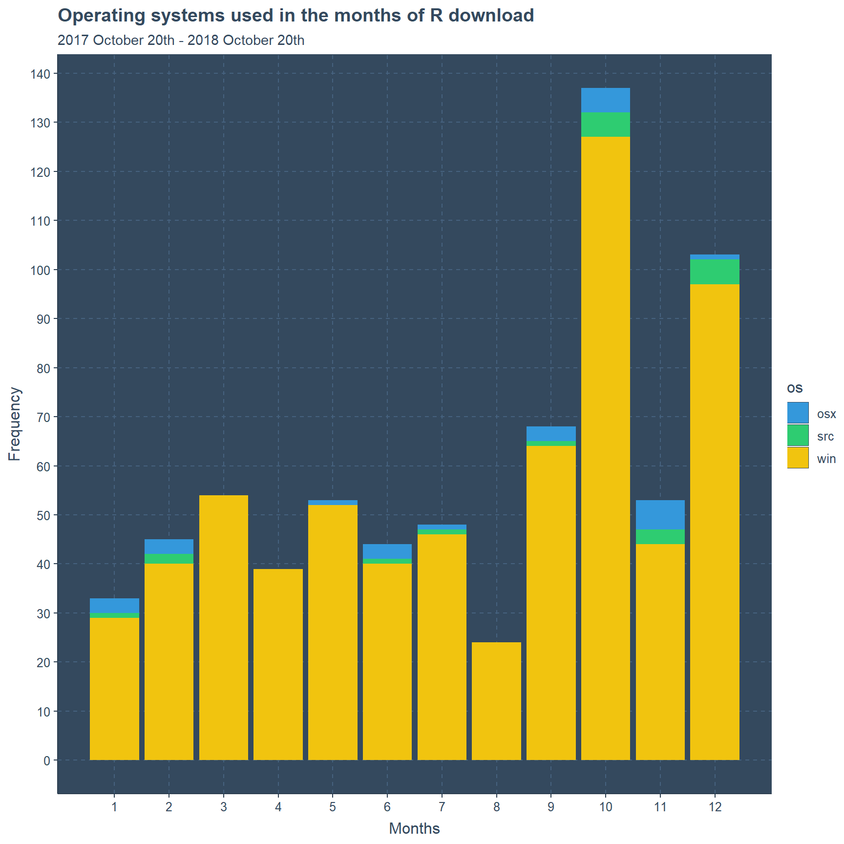
So, the first sub part of time is months. Here, we are considering 12 months of an year and months August and April reflects no Operating System is better than Windows property. While, August holding the least amount of downloads with slightly above frequency 20. Highest frequency occurs to October with count higher than 130 and significantly osx and src types of files also have higher amount than any-other month. Except August only the month of December has counts higher than 100.
#checking which days the downloads occured inrespecitive to operating system
ggplot(r_downloads_year_LK,aes(x=day(date),fill=os))+
    geom_bar()+xlab("Days") +ylab("Frequency")+
    scale_y_continuous(breaks =seq(0,80,10))+
    scale_x_continuous(breaks=1:31)+
    ggtitle("Operating systems used in the days of R download",
              subtitle = "2017 October 20th - 2018 October 20th")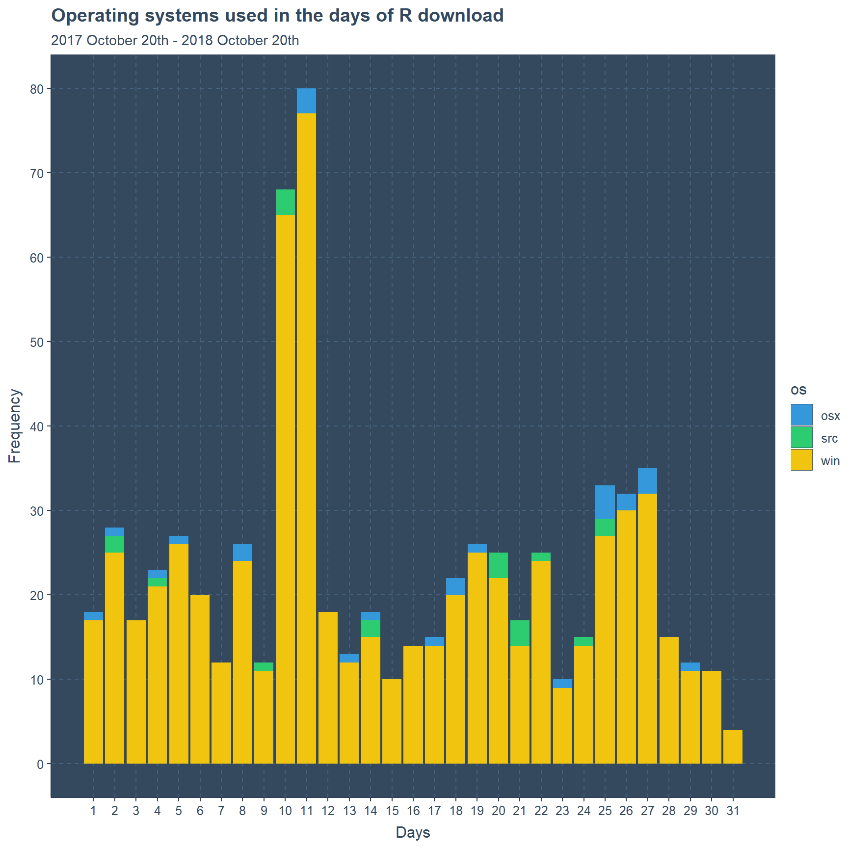
Next, focusing on the days it is clear that 10th and 11th have most downloads respectively reaching more than 60 and 70 in counts, while in other days it is mostly less than 30. Further, clearly on the 31st it includes least frequency of 10 because 31st is not a common day of all 12 months. It would be very tiring to focus on operating systems individually, but to be fair there is clear sign of few days with only the use of windows, and a few days with combination of other operating systems with windows.
#checking which hour the downloads occured inrespecitive to operating system
ggplot(r_downloads_year_LK,aes(x=hour(time),fill=os))+
    geom_bar()+xlab("Hour") +ylab("Frequency")+
    scale_y_continuous(breaks = seq(0,100,5))+
    scale_x_continuous(breaks=0:23)+
    ggtitle("Operating systems used in the Hours of the day of R download",
              subtitle = "2017 October 20th - 2018 October 20th")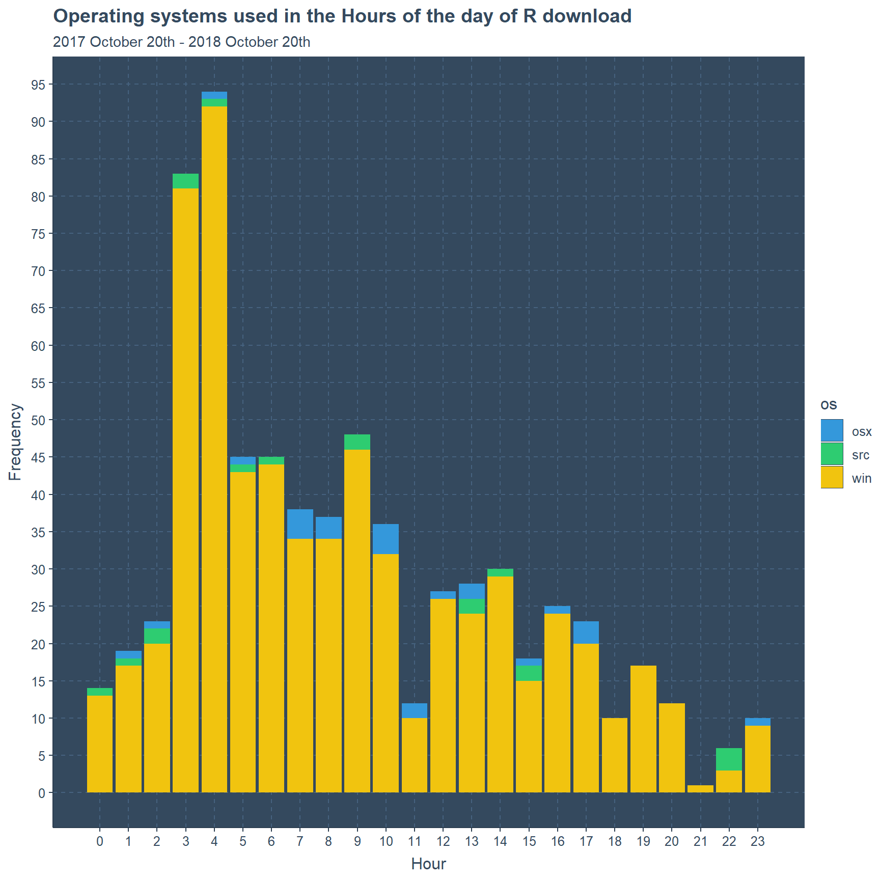
I have been curious at this part because of wanting to know at which hour of the day did our Sri Lankan users download R and packages. Yet it should be noted that the hour of time could be local time of Sri Lanka or otherwise. Still according to the bar chart the hours 4th and 5th have most downloads with counts of above 80 and above 90 respectively. Where in the 21st hour it reaches the least amount of less than 5 counts. Most of the frequencies are in the range of 10 and 35.
#checking which minute the downloads occured  inrespecitive to operating system
ggplot(r_downloads_year_LK,aes(x=minute(time),fill=os))+
    geom_bar()+xlab("Minute") +ylab("Frequency")+
    scale_y_continuous(breaks = 0:25)+
    scale_x_continuous(breaks=0:59)+
    ggtitle("Operating systems used in the minutes of the day of R download",
              subtitle = "2017 October 20th - 2018 October 20th")+
    coord_flip()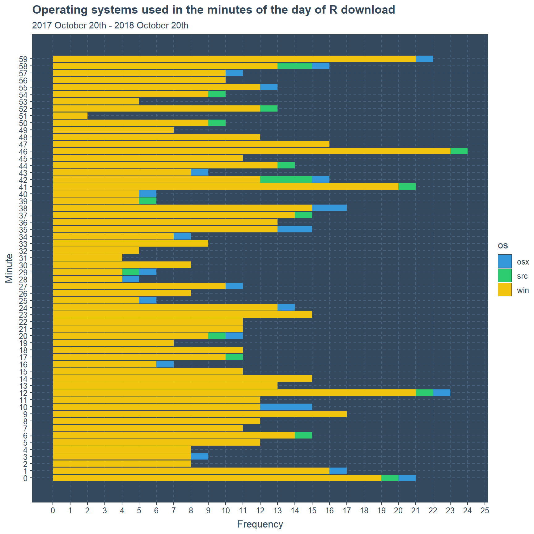
Looking at the minutes it is very spread out. Focusing on special occasions only four minutes which are 59th, 46th, 12th and 0th have counts more than 20. While 51st minute has a count of 2. Rather than this nothing more significant occurs here. I think considering these counts in perspective of specific operating systems is tedious amount of work and waste of time.
Download Size and IP ID
Packages were downloaded but none of their names were given in this data-set. Therefore we cannot know which package were downloaded. Yet we can identify the package sizes which were downloaded most. According to the table an R package with 82375220 bytes has most downloads of 50, while second place goes to to a size of 82375219 bytes and finally in third place is for 82375216 bytes with 39 counts.
# table of frequency for sizes of download
tab3<-as.data.frame(sort(table(r_downloads_year_LK$size))%>% tail(5))
names(tab3)<-c("Size","Frequency")
kable(tab3)  %>%
  kable_styling(bootstrap_options = "striped", full_width = F,position="left") %>%
add_header_above(c("Frequency table to Download size"=2))| Size | Frequency |
|---|---|
| 82877772 | 18 |
| 78171328 | 22 |
| 82375216 | 39 |
| 82375219 | 48 |
| 82375220 | 50 |
Looking at the IP ID it is clear that 334 has the highest downloads of 55, while second place goes to 1060 with 46 downloads. Finally, ID number 1286 has 16 downloads with third place.
# table of frequency to IP ID
tab4<-as.data.frame(sort(table(r_downloads_year_LK$ip_id))%>% tail(5))
names(tab4)<-c("IP ID","Frequency")
kable(tab4)  %>%
  kable_styling(bootstrap_options = "striped", full_width = F,position="left") %>%
add_header_above(c("Frequency table to IP ID"=2))| IP ID | Frequency |
|---|---|
| 623 | 9 |
| 157 | 12 |
| 1286 | 16 |
| 1060 | 46 |
| 334 | 55 |
Conclusion
I shall conclude my findings in point form
Most of Sri lankans (93.58%) use windows as a OS for R downloads
Top three R versions are 3.5.1, 3.4.3 and 3.5.0 with percentages respectively 36.52% 27.96% and 15.98%.
Windows users use versions 3.5.1, 3.4.3 and 3.5.0 with percentages 34.56%, 26.53% and 3.5.0.
Most of the downloads occur in the months October and December, while days are 10th and 11th, while hours are 3rd and 4th and minutes of 59th, 46th, 12th and 0th.
Download size of 82375220 bytes happens with the highest count of 50, while the IP ID of 334 has most downloads of 55.
Further Analysis
We can do similar analysis for other countries and compare them.
Using Size it should be possible to understand what is being downloaded.
Please see that
This is my Second post on the internet so please be kind to tolerate my mistakes in grammar and spellings. I intend to post more statistics related materials in the future and learn accordingly. Thank you for reading.
THANK YOU