# load the necessary packages
library(tidyverse)
library(lubridate)
library(kableExtra)
library(ggthemr)

#load the ggthemr
ggthemr("flat dark")

# load the data set
tidytuesday_tweets<-readRDS("tidytuesday_tweets.rds")
#Tidytuesday Tweets
Using plots and Tables to express the #TidyTuesday data-set. You can obtain the dataset from here.
Favorite count vs Retweet count. Code: https://t.co/QJwXxzrkFG
— Amalan Mahendran (@Amalan_Con_Stat) January 1, 2019
#TidyTuesday #tidyverse pic.twitter.com/l14pHDS3kq
Earliest Tweet
The first tweet is on April 2nd and it has 156 favorites and 64 retweets, where the tweet is from Thomas Mock and the next 3 tweets are also from him.
tidytuesday_tweets[order(tidytuesday_tweets$created_at),c(3,4,13,14,71)] %>%
  head(5) %>%
  kable()  %>%
kable_styling()| created_at | screen_name | favorite_count | retweet_count | name |
|---|---|---|---|---|
| 2018-04-02 21:35:08 | thomas_mock | 156 | 64 | Thomas Mock |
| 2018-04-02 21:35:10 | thomas_mock | 6 | 0 | Thomas Mock |
| 2018-04-02 21:35:11 | thomas_mock | 4 | 0 | Thomas Mock |
| 2018-04-02 23:31:11 | thomas_mock | 2 | 0 | Thomas Mock |
| 2018-04-03 00:25:51 | umairdurrani87 | 6 | 2 | Umair Durrani |
Any Verified Profiles ?
There are only 3 verified profiles where Hadley Wickham has the highest amount of followers with 76469, where that tweet has 61 favorites but no retweets. Other profiles are Civis Analytics and grspur, but both of them have friends above 600 counts, but Hadley Wickham friends count is close to 290.
subset(tidytuesday_tweets[,c(4,13,14,76,77,82)],verified==TRUE) %>%
  kable() %>%
kable_styling()| screen_name | favorite_count | retweet_count | followers_count | friends_count | verified |
|---|---|---|---|---|---|
| CivisAnalytics | 3 | 1 | 6880 | 658 | TRUE |
| hadleywickham | 61 | 0 | 76469 | 288 | TRUE |
| grspur | 14 | 6 | 857 | 623 | TRUE |
Source of Tweets
Close to 1050 tweets are done by the web client and other clients such as Android and Iphone have tweet counts of respectively 106 and 233. Other sources include oddly Instagram, Facebook, WordPress and LinkedIn, which I am naming because of their popularity.
ggplot(tidytuesday_tweets,aes(fct_infreq(source)))+
  geom_bar()+coord_flip()+
  geom_text(stat = "count",aes(label=..count..),hjust=-0.25)+
  ylab("Frequency")+xlab("Types of Sources")+
  ggtitle("Source of Tweets")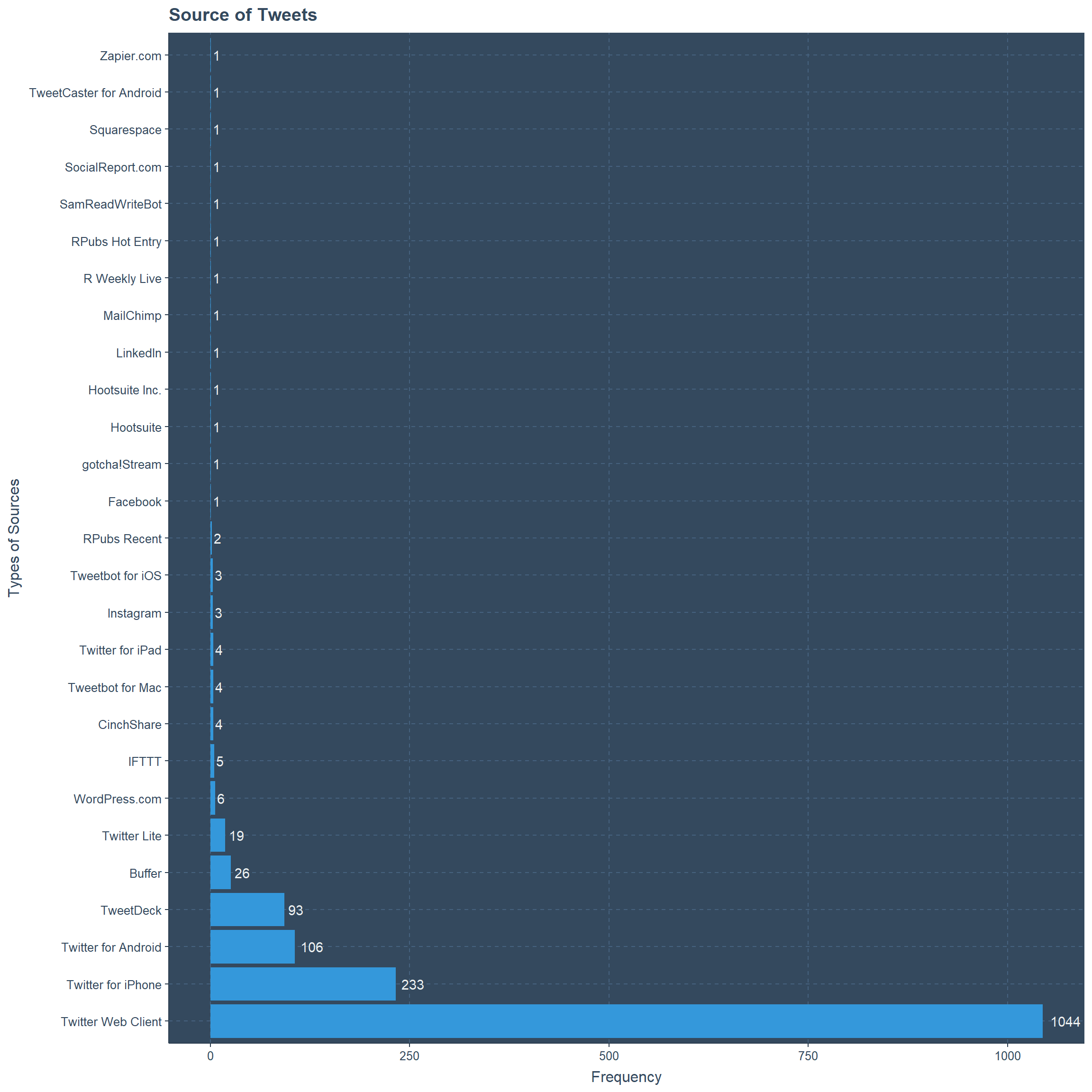
Tweets Per Month
Beginning of #TidyTuesday we have 293 tweets on the month of April. Even though over the next months the number of tweets are decreasing this is not the case in October. Lowest number of tweets are recorded in September with 115 tweets.
ggplot(tidytuesday_tweets,
       aes(x=month(tidytuesday_tweets$created_at)))+
  geom_bar()+
  geom_text(stat = "count",aes(label=..count..),vjust=-0.15)+
  scale_x_continuous(breaks = seq(1,12),labels = seq(1,12))+
  ylab("Frequency")+ xlab("Months")+
  ggtitle("Tweet Counts By Month")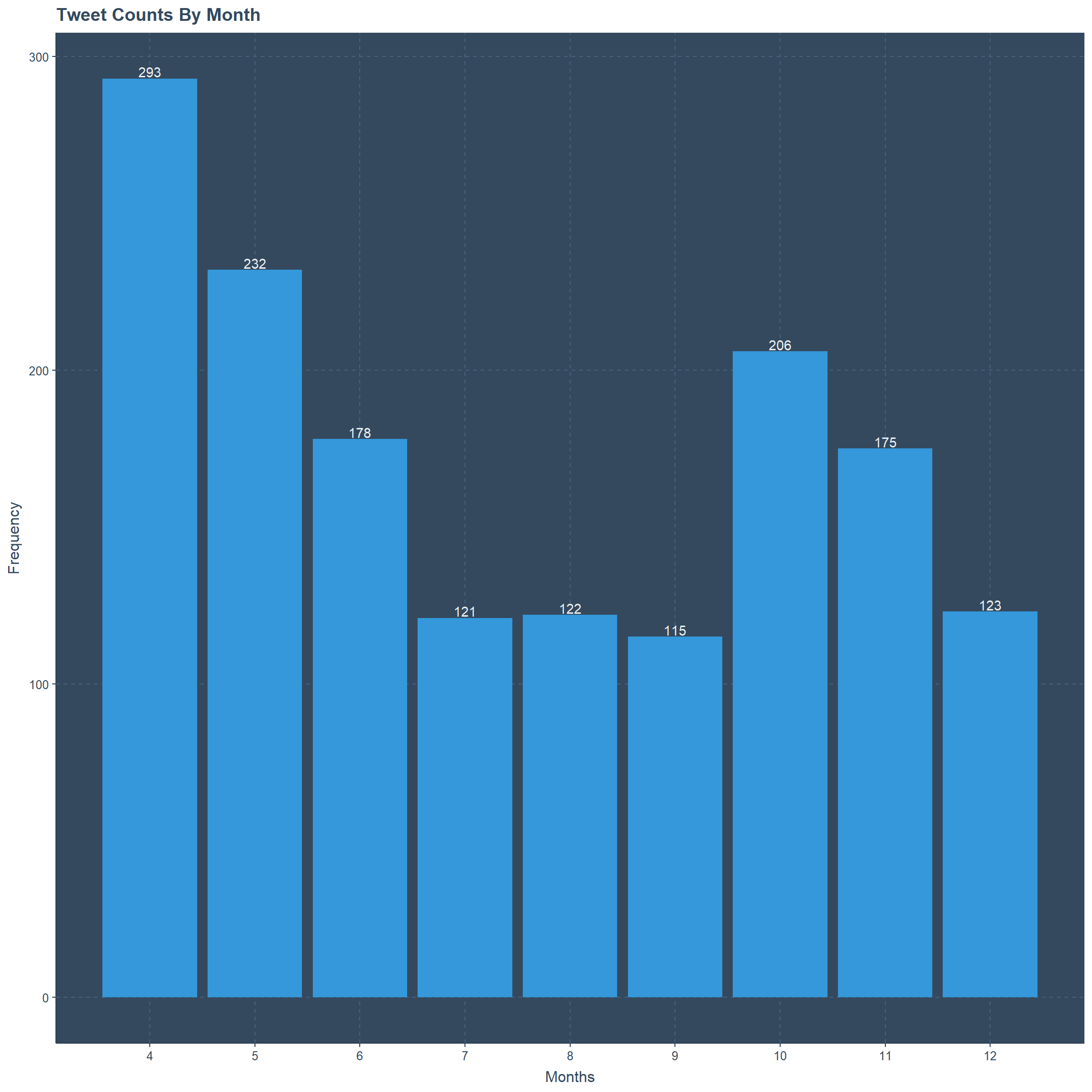
Most Tweets By Screen Name
There are 30 twitter users if we consider the accounts that have tweeted more than or equal to 10 tweets under the hashtag “TidyTuesday”. Thomas Mock has tweeted most which is 172 including retweets, and the second place goes to R4DScommunity with 92 tweets. All the other users have individually less than 40 tweets.
tidytuesday_tweets %>%
  group_by(screen_name) %>%
  filter(n() >= 10) %>%
ggplot(aes(x=fct_infreq(screen_name)))+
  geom_bar()+ coord_flip()+
  geom_text(stat = "count",aes(label=..count..),hjust=-0.15)+
  ylab("Frequency")+ xlab("Screen Name")+
  ggtitle("Screen Name with Most Tweets")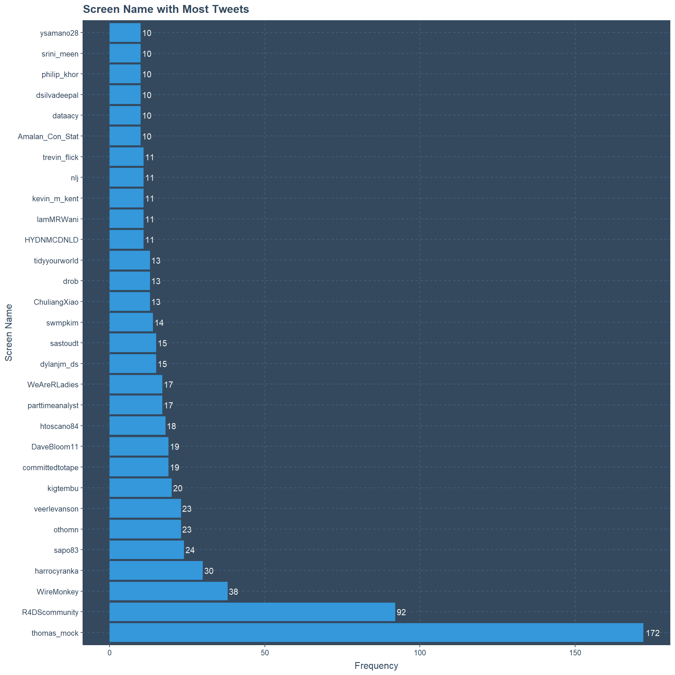
Most Tweets By Screen Name and their Source
For the same plot if we consider the source for the tweets, it is clear that only seven sources were used. Mostly all of these users are using the web client, but some are using the iPhone as well. R4DS community does more tweeting through iPhone than TweetDeck. TweetDeck is a simple way of handling multiple twitter accounts at the same time. Tidyyourworld account only uses Android and WeAreRLadies uses only TweetDeck.
tidytuesday_tweets %>%
  group_by(screen_name) %>%
  filter(n() >= 10) %>%
ggplot(aes(x=fct_infreq(screen_name),fill=source))+
  geom_bar(position = "stack",stat="count")+
  coord_flip()+
  geom_text(stat = "count",aes(label=..count..),hjust=1,
            position = position_stack())+
  ylab("Frequency")+ xlab("Screen Name")+
  ggtitle("Screen Name with Most Tweets and their Source")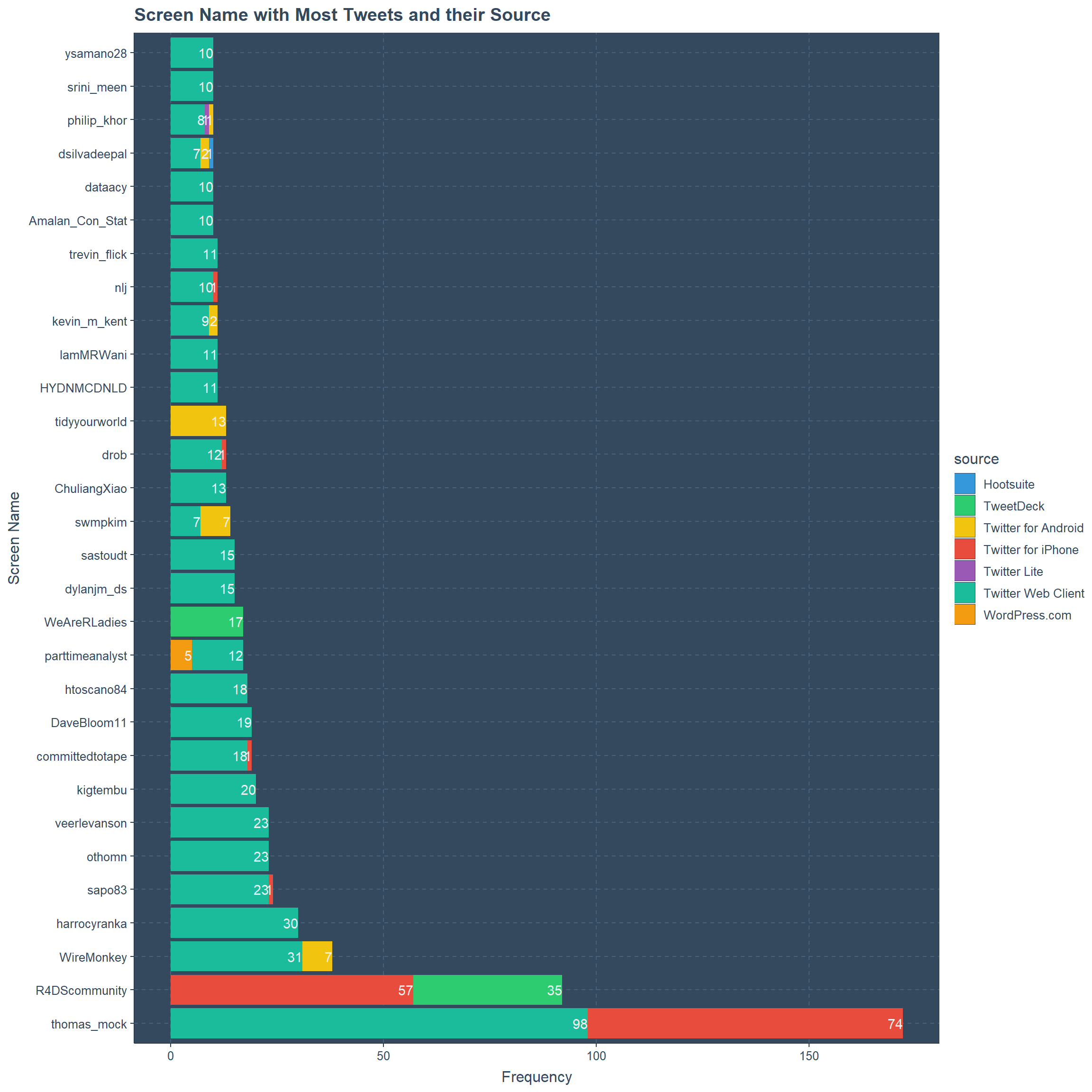
Most Tweets By Screen Name with their Retweet Counts
Of the Top 30 users with most amount of tweets the highest amount of retweets is to a tweet from WeAreRLadies and it is 95. There are more outliers from Thomas Mock. and the highest range is to the user drob. Most from this top 30 users have the range between 0 and 10.
tidytuesday_tweets[,c("screen_name","retweet_count")] %>%
  group_by(screen_name) %>%
  filter(n() >= 10) %>%
ggplot(.,aes(x=fct_infreq(screen_name),y=retweet_count))+
  geom_boxplot()+ coord_flip()+
  scale_y_continuous(breaks = seq(0,100,5),labels = seq(0,100,5))+
  ylab("Retweets")+ xlab("Screen Name")+
  ggtitle("Screen Name with Most Tweets and their Retweets Count")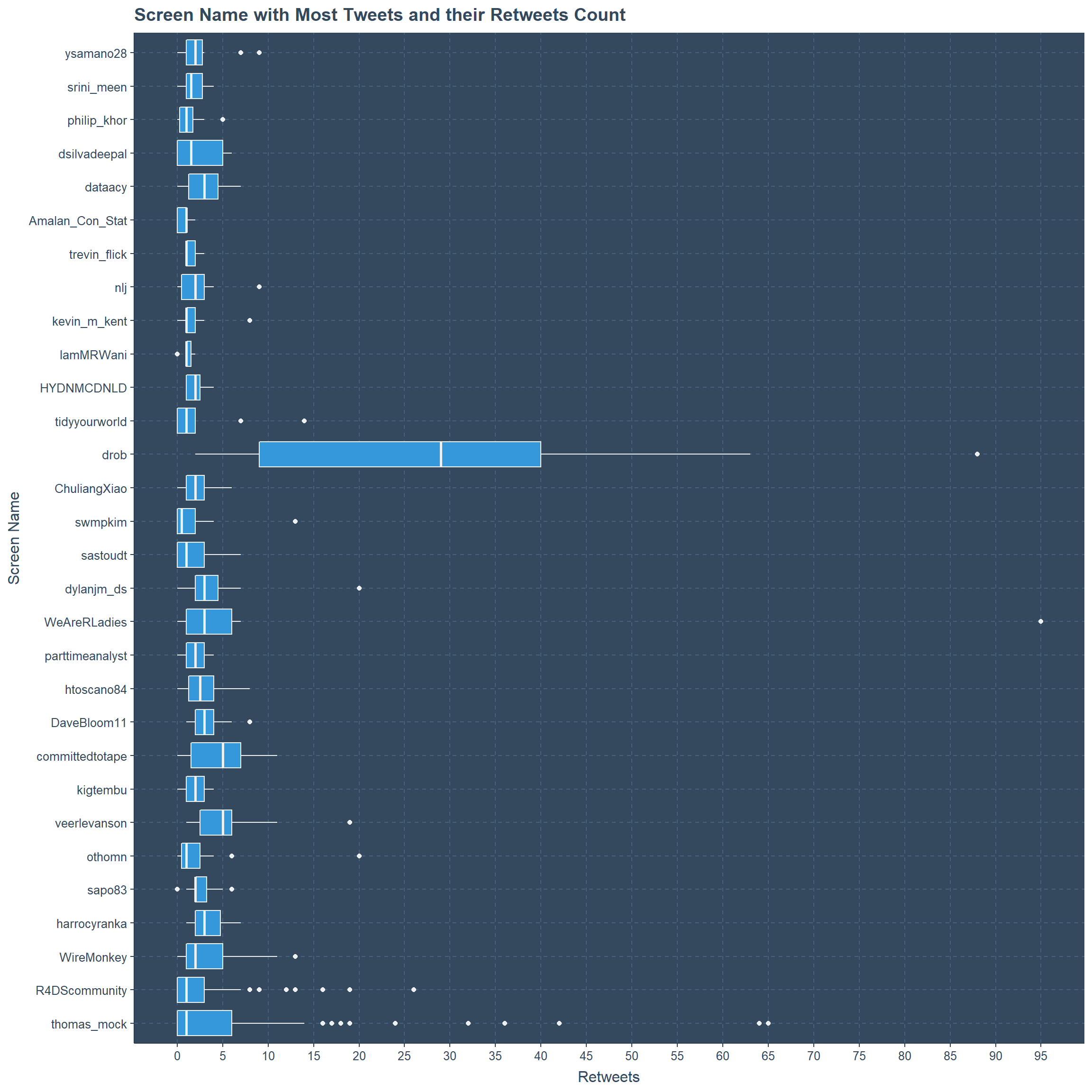
Most Tweets By Screen Name with their Favorite Counts
Similarly Thomas Mock has more outliers, and the highest range is to the user drob. Second place for outliers goes to R4DScommunity user. Close to 500 favorites are counted to a tweet by drob and second place is to a tweet by WeAreRladies with favorite counts slightly above 450.
tidytuesday_tweets[,c("screen_name","favorite_count")] %>%
  group_by(screen_name) %>%
  filter(n() >= 10) %>%
ggplot(.,aes(x=fct_infreq(screen_name),y=favorite_count))+
  geom_boxplot()+ coord_flip()+
   scale_y_continuous(breaks = seq(0,500,25),labels = seq(0,500,25))+
  ylab("Favourites Count")+ xlab("Screen Name")+
  ggtitle("Screen Name with Most Tweets and their Favourties Count")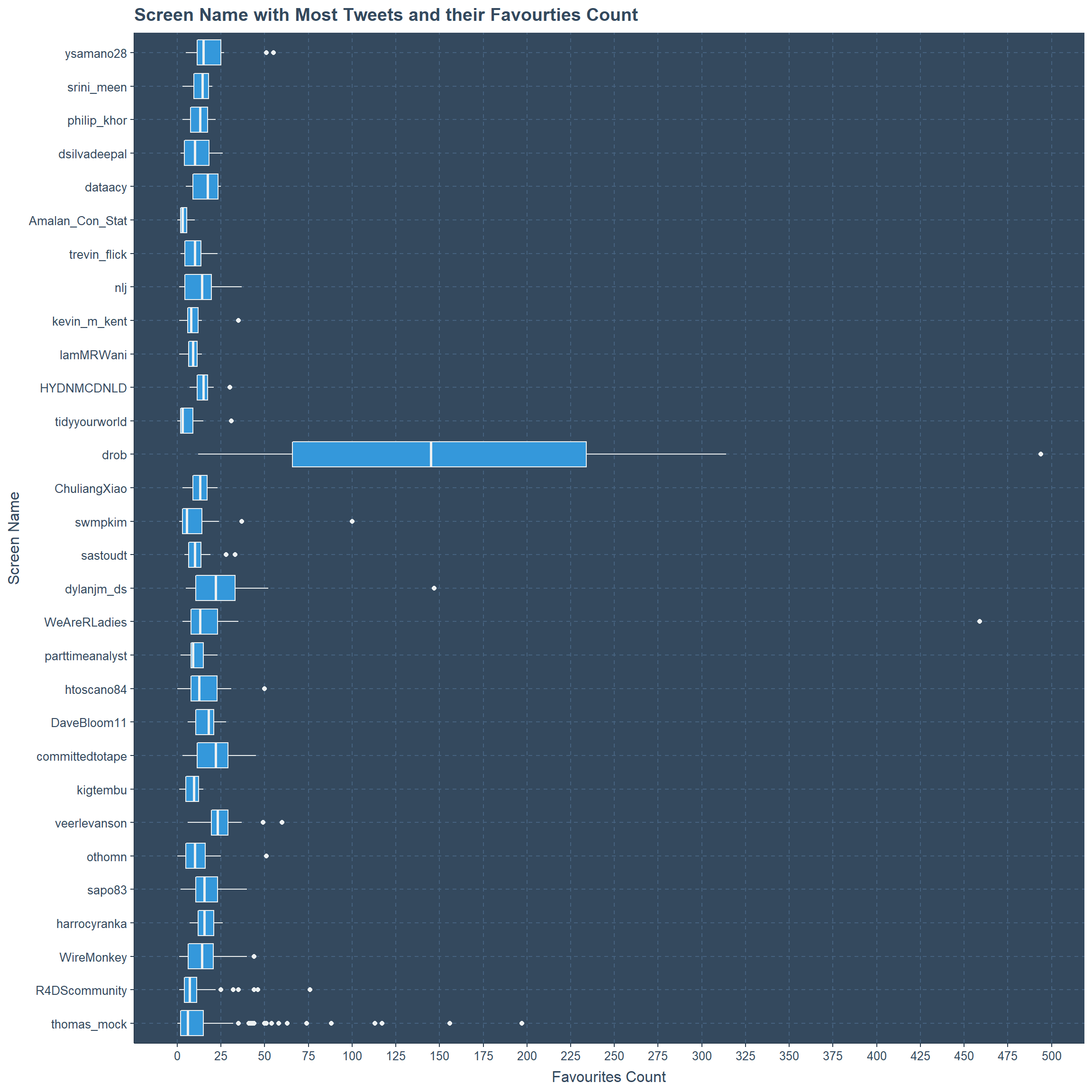
Relationship between Favorite Counts vs Retweet Counts ?
Very clear positive correlation. Y scale ranges from 0 to 500, where x scale range is from 0 to 100 and most of the data points are centered around the range of 0 to 12 retweets and 0 to 60 Favorites. A Few data data points are out of the above mentioned range.
ggplot(tidytuesday_tweets,
       aes(x=retweet_count,y=favorite_count))+
  geom_point()+geom_smooth()+
  scale_x_continuous(breaks =seq(0,100,2) ,labels =seq(0,100,2))+
  scale_y_continuous(breaks =seq(0,500,10),labels =seq(0,500,10))+
  xlab("Retweets")+ylab("Likes")+
  ggtitle("Retweets Versus Likes")
Relationship between Followers Count vs Friends Count ?
Here I have considered only twitter profiles which has followers count less than 5000 with friends count also less than 5000. The reason is to explain the relationship more clearly. Clearly most of the twitter profiles are having followers less than 2000 with friends also less than 2000. Clearly there are some profiles with Followers count above 1000 but friends count less than 1000. Even though there are few profiles with less than 1000 followers but more than 1000 Friends.
ggplot(subset(tidytuesday_tweets,
       followers_count < 5000 & friends_count < 5000),
       aes(x=followers_count,y=friends_count))+
  geom_point()+geom_smooth()+
  scale_x_continuous(breaks =seq(0,5000,250),labels =seq(0,5000,250))+
  scale_y_continuous(breaks =seq(0,5000,250),labels =seq(0,5000,250))+
  xlab("Followers Count")+ylab("Friends Count")+
  ggtitle("Followers Count Versus Friends Count")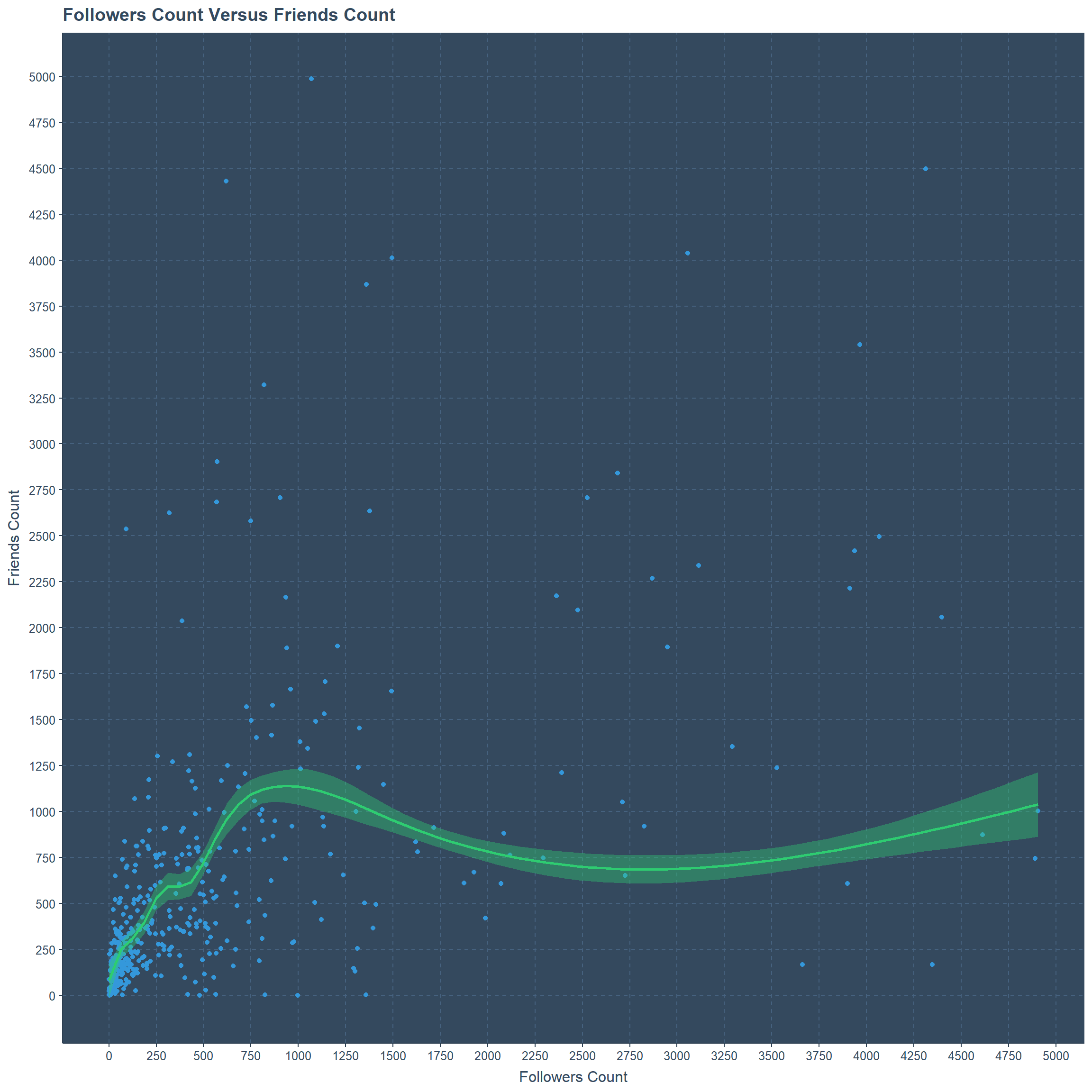
Conclusion
My conclusion of the above plots and tables in point form
Using tidyverse as usual is fun.
The Box plots for several variables in the same plot is easy for the use of comparison.
The Scatter plots are nice to understand the relationship among two continuous variables.
The geom_smooth function is also very useful in modelling the data.
Further Analysis
We can focus on the text variable which could be used for a word cloud.
Further we can try to understand the hashtags with favorites and retweets.
THANK YOU