
Data is for Week 43 under the title Horror Movies. Have not done any plotting for TidyTuesday for some time or to be exact more than two months. So here I am trying out d3 visualisation in R.
Helpful packages for this post are ‘d3rain’ and ‘d3treeR’.
# load the packages
library(d3rain)
library(dplyr)
library(ggplot2)
library(splitstackshape)
library(d3treeR)
library(treemap)

# load the data
horror_movies <- readr::read_csv("https://raw.githubusercontent.com/rfordatascience/tidytuesday/master/data/2019/2019-10-22/horror_movies.csv")
Organize Data
Genuine look indicates that data is fine. Well if you look closer there are some changes that need to be done to make the most of it. I have simpler dreams such as drawing two plots which would make sense.
Rain plot where Horror movie distribution occurs by each month for days.(Easier to look at the plot than try to grasp from what I am telling)
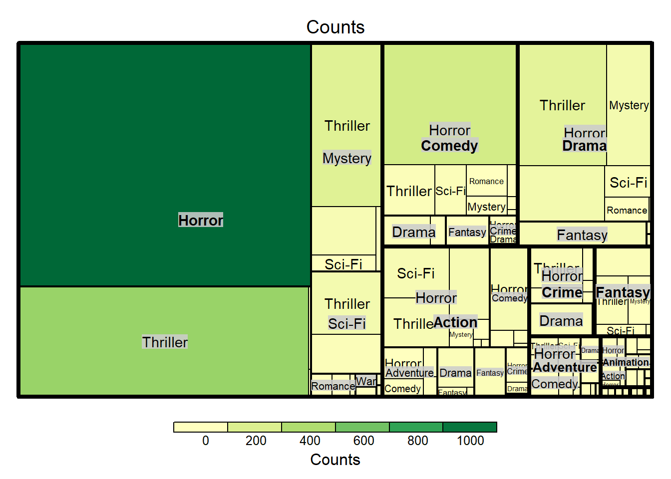
Tree map which would indicate how the Genres of the movies are assigned. It is my intention to understand if there is a hierarchy in this genre naming as some movies have multiple assignments.
To achieve above set plots some changes in the two columns ‘genres’ and ‘release_date’ are necessary; precisely we have to break one column into multiples based on a pattern for former and based on a condition for latter.
RainDataFormat <- cSplit(horror_movies,'release_date','-',drop=TRUE)

RainDataFormat <- RainDataFormat %>%
                    rename(Day = release_date_1) %>%
                    rename(Month = release_date_2) %>%
                    rename(Year = release_date_3) %>%
                    select(Year,Month,Day,title)

RainDataFormat$Year[is.na(RainDataFormat$Year)==TRUE] <-
    stringr::str_remove(RainDataFormat$Day[is.na(RainDataFormat$Year)==TRUE],"20")

class(RainDataFormat$Year) <- "numeric"
class(RainDataFormat$Day) <- "numeric"

RainDataFormat$Day[RainDataFormat$Day>31] <- NA
TreeDataFormat <- cSplit(horror_movies,'genres','|',drop=TRUE)
TreeDataFormat <- TreeDataFormat %>%
rename(First_Choice = genres_1) %>%
rename(Second_Choice = genres_2) %>%
rename(Third_Choice = genres_3)
TreeDataFormat <- TreeDataFormat %>%
group_by(First_Choice,Second_Choice,Third_Choice) %>%
mutate("Counts" = n()) %>%
select(First_Choice,Second_Choice,Third_Choice,Counts) %>%
unique()Rain Graph
Compared how horror movies have increased compared to year 2017 from year 2012.
RainDataFormat <- RainDataFormat[complete.cases(RainDataFormat)]
levels(RainDataFormat$Month) <- c("Jan","Feb","Mar","Apr",
                                  "May","Jun","Jul","Aug",
                                  "Sep","Oct","Nov","Dec")

RainDataFormat[Year==12] %>%
    d3rain(Day,Month,toolTip = Day,title = "Days vs Months for Year 2012") %>%
    drip_settings(dripSequence = 'iterate',
                  ease = 'linear',
                  jitterWidth = 25,
                  dripSpeed = 500,
                  dripFill = 'steelblue') %>%
    chart_settings(fontFamily = 'times',
                   yAxisTickLocation = 'left')
RainDataFormat[Year==17] %>%
d3rain(Day,Month,toolTip = Day,title = "Days vs Months for Year 2017") %>%
drip_settings(dripSequence = 'iterate',
ease = 'linear',
jitterWidth = 25,
dripSpeed = 500,
dripFill = 'red') %>%
chart_settings(fontFamily = 'times',
yAxisTickLocation = 'left')Tree map
Some movies have more than three genres assigned to them. So here is the tree map to plot them in choice order for genre.
TreeData <- treemap(
                    TreeDataFormat,
                    index=c("First_Choice", "Second_Choice",'Third_Choice'),
                    vSize="Counts",
                    vColor="Counts",
                    type="value"
                    )

d3tree3(TreeData,rootname = "Choices")
THANK YOU